When defining coverage items we need to make a trade-off between the number of coverage buckets, their size and the simulation time required to get them covered. From our experience the solution is to generate items being aware of how they will be covered. For example if the coverage item has power-of-2 buckets, the generated items should not follow a flat distribution. A distribution that guarantees more hits for the smaller intervals and less hits for the larger intervals makes more sense.
This article illustrates a new way of optimizing stimulus generation in order to get faster coverage closure by using e Language features supported by Cadence tools.
Covering Bus Connectivity
If you want to verify the connectivity over a bus or make sure large data paths have been toggled enough, you can either use bit toggling buckets or define more buckets/ranges for the bus value. Sampling all zeros and all ones easily covers all the bit toggling buckets, thus the second option is usually preferred, as it gives more confidence that there is enough activity on the bus. One way to partition the valid space is using power-of-2 intervals:
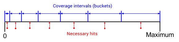
Power-of-2 coverage intervals are uneven and covering the smaller bins takes a lot of time when using flat distribution generation. In large projects, tweaking generation and adding directed test cases to get these buckets filled 100% may take weeks of regressions time.
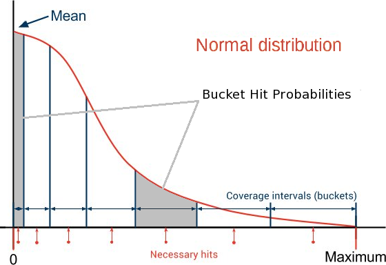
The solution is to generate items using a distribution that guarantees more hits when closer to 0 and less hits when closer to the maximum value. Overall, all buckets get the same chance to be hit/filled, even though one bucket may contain only one value, while other buckets may contain thousands.
Normal Distribution
Starting with INCISIVE 13.1 Cadence introduced a new way of constraining the generation of items. You can now generate items with normal distribution and even control the shape of the Bell Curve. It is now possible to generate items that will quickly fill power-of-2 intervals. You can do it by adding a single constraint:
data : uint;
keep data in [MIN_VAL..MAX_VAL];
keep soft data == select {
    100 : normal(MEAN, SIGMA);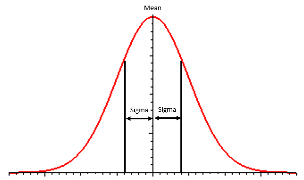
};- MEAN is the location of the peak;
- SIGMA is the interval [MEAN..(MEAN±SIGMA)]) where 66% of the numbers will be generated.
You can see the constrained distribution in the picture below.
Example
I created a small example to test the new feature. The code defines an uint field data which is constrained inside a [MIN_VAL..MAX_VAL] interval. MIN_VAL will always be 0 while MAX_VAL will be different powers-of-2 values. Data is generated and then covered using a macro which splits the coverage interval into power-of-2 buckets.
The new normal distribution constraint can be seen below.
<'
// Adjust FACTOR to get the slope you are looking for.
// For power-of-2 coverage intervals FACTOR should decrease as (MAX_VAL - MIN_VAL + 1) increases.

import cover_data_macro;

define MAX_POWER_OF_TWO 12;

define MIN_VAL 0;
define MAX_VAL ipow(2, MAX_POWER_OF_TWO) - 1;

// FACTOR determines the shape of the Bell Curve.
define FACTOR  0.15;
// SIGMA is computed by multiplying the data interval size with FACTOR.
define SIGMA   (MAX_VAL-MIN_VAL+1) * FACTOR;

define MEAN     MIN_VAL;

extend sys  {
   data : uint;
   keep data in [MIN_VAL..MAX_VAL];
   keep soft data == select {
      //Inside the select brackets you define the weight (100),
      //the type of distribution (normal), the peak of Bell Curve (MEAN),
      //and the standard deviation (SIGMA).
      //Within the standard deviation interval 66% of the values will be generated.
      100: normal(MEAN, SIGMA);
   };

   event data_cvr_e;
   cover data_cvr_e is {
      cover_data MAX_POWER_OF_TWO
   };
   run() is also {
      for i from 0 to 1000 {
         gen data;
         emit data_cvr_e;
      };
   };
};
'>
As there are many small buckets to cover closer to zero, the code above generates smaller values with higher probability in order to compensate for smaller bucket size closer to zero:
For example a 12 bits constraint “translates” to:
data : uint (bits : 12);
keep soft data == select {
    100 : normal(0, ipow(2, 12)*0.15);
};
and this is the distribution of samples after 1001 generations:
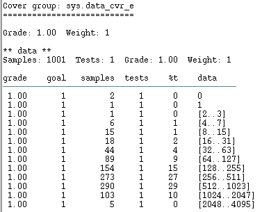
For 12 bits setting the MEAN to 0 and computing SIGMA as ipow(2, 12)*0.15 fairly distributes the necessary hits.
Flat Distribution vs. Normal Distribution
The chart below shows the difference between flat and normal distribution for a 12 bits bus. It can be easily seen that most of the generated values are near 0 for the normal distribution. For a clearer view, each point on the graph represents the number of samples in a bin of 20 values.
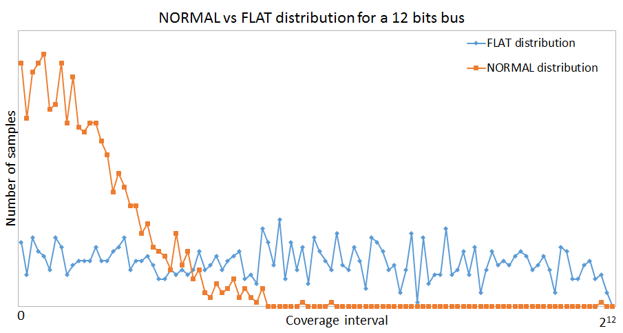
For the next coverage examples I used the same code as above, I just removed the normal generation constraint to get a flat distribution.
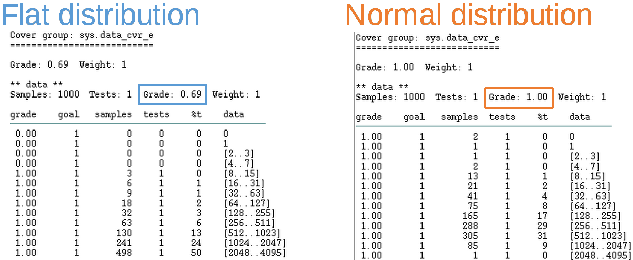
Covering [0..212] in 1_000 samples.
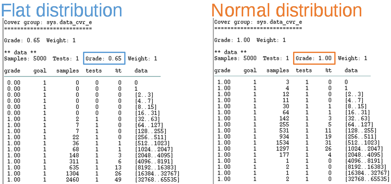
Covering [0..216] in 5_000 samples.
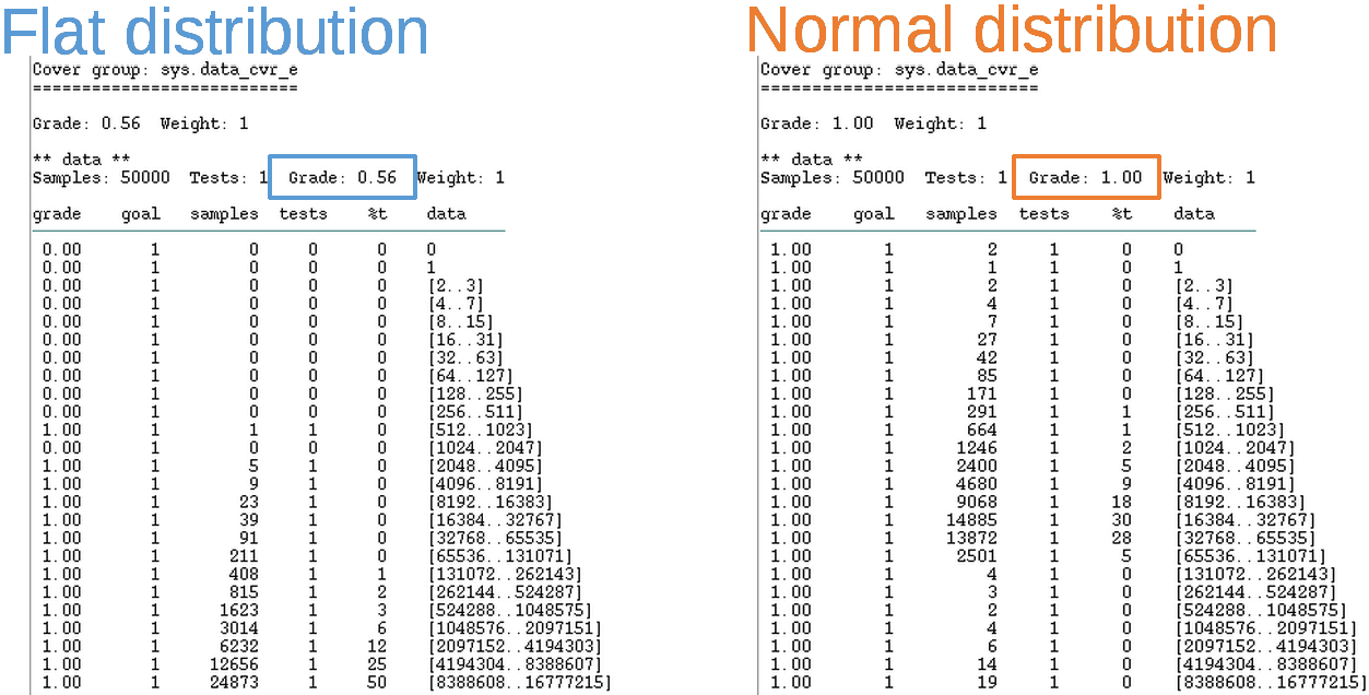
Covering [0..224] in 50_000 samples.
How to Choose the Right Value for FACTOR?
The only unknown is the FACTOR that controls the shape of the distribution.
data : uint (bits : 16);
keep soft data == select {
    100 : normal(0, ipow(2, 16) * FACTOR);
};
You should start with some value and tune it across a couple of “experimental” generation iterations in order to get “the right shape” that fills the buckets using an acceptable number of samples. Too few means not exercised enough. Too many means too redundant (and expensive).
For example, some possible values for FACTOR, empirically computed for different interval sizes can be seen below.
|
Interval |
FACTOR | Samples required for 100% coverage |
|
[0..24] |
0.4 | 10 |
|
[0..28] |
0.2 |
100 |
|
[0..212] |
0.15 |
1_000 |
| [0..216] | 0.02 |
5_000 |
| [0..220] | 0.015 |
15_000 |
| [0..224] | 0.0018 |
50_000 |
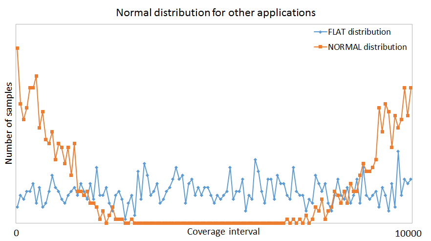
Other Applications
If you have a coverage item that splits the coverage interval into three areas of interest: minimum values, maximum values and anything in between; you can also improve generation by using the above technique.
In this case you can use two normal distribution constrains each with a 50% chance of generating values. The generation engine will then hit more values when reaching the borders of the coverage interval and less in the middle.
This proved to be very useful in one of the projects I worked on as it helped us find a bug that was triggered by multiple apparently unrelated counters wrapping around at the same time.
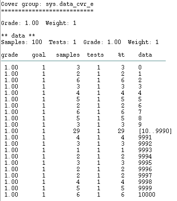
The following code covers the three intervals in 100 samples:
<'
extend sys {
    data : uint;
    keep data <= 10000;
    keep soft data == select {
        50 : normal(0,     10000*0.001);
        50 : normal(10000, 10000*0.001);
    };
    event data_cvr_e;
    cover data_cvr_e is {
        item data using ranges = {
            range ([0..9],        "", 1);
            range ([10..9990]);
            range ([9991..10000], "", 1);
        };
    };
    run() is also {
        for i from 1 to 100 {
            gen data;
            emit data_cvr_e;
        };
    };
};
'>
And this is how the two normal distribution look when plotted on a chart. For a clearer view, each point on the graph represents the number of samples in a bin of 8 values.
Conclusions
Non-uniform generation is extremely useful and can gain a project:
-
Regression saving: less resources (time, CPU…) are spent on running thousands of tests in order to cover exotic intervals and values
-
Time saving: less time and manpower are spent in analyzing coverage and writing directed tests to cover these hard to hit values