The process of generating a higher resolution image from a low resolution image, requires identifying the missing pixels. This filling-in of the “pixel gaps” has been addressed by various machine learning methods. From the variety of methods, convolutional neural networks stand out, due to their reusability and their small number of parameters. Taking advantage of the hierarchical structure of the data in the images, an implementation of CNN at the level of reconfigurable hardware can significantly exceed the time performance offered by most general purpose processing units.
This article describes the techniques used to accelerate an image upscaling convolutional neural network on an FPGA using high-level synthesis (HLS). The acceleration was done using a real-time encoding style and various optimization techniques, with a negligible impact on image quality at super-resolutions. To emphasize the results, I used the bicubic interpolation algorithm as a reference. I analyzed and compared the performance profiles of the implemented accelerators both on an FPGA (Xilinx – Zynq-7000 SoC), and on a standard x64 CPU (Intel Core i5-6200U).
Table of Contents
- What is Image Upscaling?
- Why Use an FPGA?
- Why Use HLS?
- The Proposed Workflow
- Implemented Algorithms
- Implementation Details
- FPGA vs CPU
- Conclusion
- Reproducing the results
- Github
- Acknowledgement
What is Image Upscaling?
The image upscaling process is integrated into the daily life of each of us, to a greater or lesser extent. Many TV owners have ultra-high definition TVs. However, the content that people often try to view with popular streaming services such as HBO and Youtube is only available at low resolution. Therefore, to view full screen images, the initial content must be enlarged.
The image upscaling process is used in various applications including image editors, magnifying glass software, web browsers, but also in different embedded systems.
Why Use an FPGA?
In addition to the enhanced image quality, the execution time of the algorithm is another important factor. The CPUs which are designed for universal purposes offer low efficiency, both in terms of resources used and the time profile of the algorithm. In terms of execution time, GPUs represent a more efficient option for algorithms that process large data conglomerations in parallel. However, GPUs do not meet the physical limitations of many embedded systems. Other more feasible options may be ASICs, which involve reliability but high costs and long design time. The non-recurring engineering (NRE – researching, designing, developing and testing) cost of an ASIC can run into millions of dollars. An FPGA is more cost-efficient than an ASIC for lower production volumes or small designs. FPGAs are configurable digital integrated circuits that can be used as hardware accelerators.
Why Use HLS?
FPGA configuration is specified using a hardware description language (HDL) like VHDL or Verilog. HDL implementation of a neural network can be difficult and time consuming which is why I chose to use high-level synthesis. HLS transforms a high-level language (C ++, SystemC, OpenCL framework, Matlab) algorithm into an RTL implementation.
Seen as the foundational technology for the RTL design evolution, HLS represents a new methodology that can overcome challenges like: human productivity gap caused by the rapid increase in design complexity, the quality gap and the verification predictability gap.
The Proposed Workflow
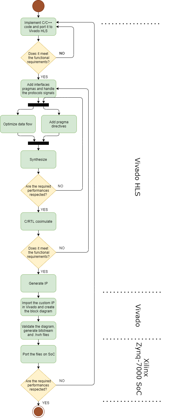
Figure 1: Workflow overview
Implemented Algorithms
The image upscaling methods I have implemented and accelerated are: the forward propagation of the FSRCNN machine learning method (Fast Super-Resolution Convolutional Neural Network) and the bicubic interpolation algorithm used as a reference for the convolutional neural network.
FSRCNN
FSRCNN is based on the following stages: feature extraction, shrinking, mapping, extension and deconvolution as illustrated in Figure 2: FSRCNN Architecture. The first four are built through convolution layers, while the last stage consists of a deconvolution layer. Deconvolution means the operation opposite to convolution.
I chose to accelerate FSRCNN considering the following characteristics:
- small number of parameters – 4036 parameters (e.g. SRCNN-Ex – is 14.16X larger than FSRCNN with 57 184 parameters);
- high image quality at super-resolution (better than SRCNN-Ex);
- high parallelization potential.
I took over the network parameters (weights, biases, PReLU parameters) from the FSRCNN article site – http://mmlab.ie.cuhk.edu.hk/projects/FSRCNN.html. This project involves implementing the forward propagation of the FSRCNN based on the model taken over and redesigning and implementing the accelerated network.
The referenced model was trained with the 91 images dataset and with General-100 dataset. Stochastic gradient descent with the standard backpropagation was used as an optimization algorithm. PReLU was chosen as an activation function to avoid zero gradients. The sensitive variables of the network were chosen by experimental method, thus: the number of mapping layers is 4, the number of extracted features from the first hidden layer is 56 and the reduced number of features obtained from the second layer is 12.
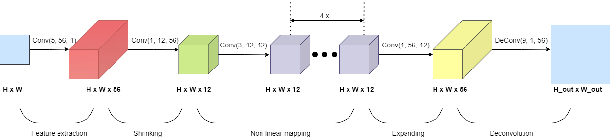
Figure 2: FSRCNN Architecture
As shown in Figure 2: FSRCNN Architecture, the referenced network has 8 layers: 7 convolutional layers and one deconvolutional layer.
| Hidden Layer | Size of the convolution filter | Number of filters / output channels | Number of input channels | Padding number | Stride |
|---|---|---|---|---|---|
| 1 | 5 | 56 | 1 | 2 | 1 |
| 2 | 1 | 12 | 56 | 0 | 1 |
| 3 | 3 | 12 | 12 | 1 | 1 |
| 4 | 3 | 12 | 12 | 1 | 1 |
| 5 | 3 | 12 | 12 | 1 | 1 |
| 6 | 3 | 12 | 12 | 1 | 1 |
| 7 | 1 | 56 | 12 | 0 | 1 |
| 8 | 9 | 1 | 56 | 1 | Upscaling factor number |
Table 1: Main parameters of the FSRCNN layers
Bicubic Interpolation
I chose this algorithm as a reference because it is widely adopted in the software world of image processing (Photoshop, Avid, Final Cut Pro and After Effects).
To perform bicubic interpolation, I applied the convolutional operation with the following kernel:
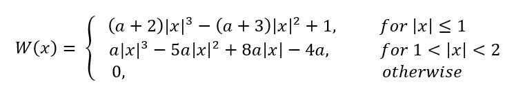
The filter is applied to the indices of 4 adjacent points in the source matrix, for each image dimension – vertical and horizontal. Thus, the inquiry pixel value is determined using the calculated weights of 16 adjacent points. The closer a source pixel is to the estimated output pixel, the greater the influence of the source pixel. Parameter a is often between -0.5 and -0.75. I chose the value of parameter a according to the results obtained by the experimental method (a = -0.5).
Implementation Details
I implemented the first versions of the algorithms (FSRCNN and bicubic interpolation) in Python in order to verify the functional correctness of the methods. I manually rewrote the entire inference step of the algorithms in C/C++. To ensure that the newly implemented C/C++ code worked fine, I tested it against the Python inference. To port the code on an FPGA using HLS, protocols must be specified for the block’s I/O ports using interface pragmas in C/C++ code. I chose AXI4-Stream protocol (AXIS) for the source image port and for the upscaled/output image port because AXIS is a simple master-slave protocol that is designed for large data transfers. Also, the lack of the address field increases the performance. For the scalar arguments of the top function (function to be synthesized) I used AXI4-Lite protocol.
Dataflow Optimization
The goal of the RTL designer is to create a programmable logic that can consume all data as soon as it reaches the interface of the block.
My Python algorithms versions have a sequential execution, running on a general purpose processor, rather than a specialized hardware. Regarding the sequential version of my FSRCNN implementation for color images (RGB standard is used), the top function stalls until it receives all of the pixels from the source image and then successively processes each color channel from the low-resolution image obtaining the high-resolution color channel. In this case, processing each input channel means passing sequentially through all levels of the network (performs first layer convolution, stalls until all of the 56 output channels from the first layer are processed, performs second layer convolution on the 56 channels and so on).
One disadvantage of the Python implementation consists in the successive processing of the input image color channels, although they are independent. Another disadvantage consists in the fact that the beginning of the execution of a layer is dependent on the completion of the execution of the previous layer. The first problem can be solved by using unroll pragma, if sufficient resources are available. The second problem can also be solved because all layers of the network are convolution/deconvolution operations and, therefore, not all data from the previous layer is needed to start computing the output response for the current layer. So, a pixel from the current layer depends on a small number of pixels from the previous layer. I solved the second problem by optimizing the data flow: I redesigned the network logic and added streams in-between the network layers to be able to apply the dataflow directive. Thus all layers of the network will concurrently process data, as it can be seen in Figure 3: FSRCNN – Data flow optimization for the blue channel.
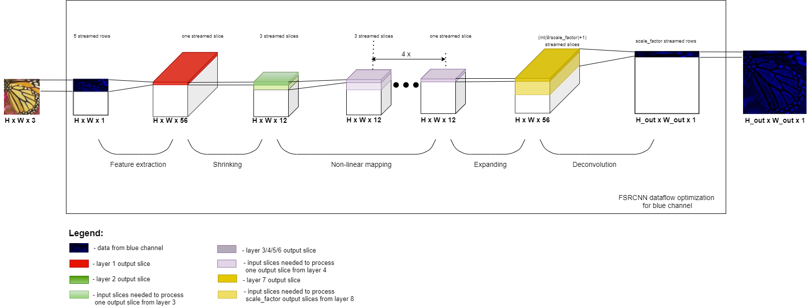
Figure 3: FSRCNN – Data flow optimization
Figure 3 suggests optimizing the data flow in order to execute operations from the next layer, without the previous one finishing its execution. Thus, as it can be seen, the first layer of the FSRCNN network (feature extraction layer) needs only 5 input blue rows of the input image to process one output slice because the size of the convolution filter of layer 1 is 5×5. Also, to process one output slice from layer 2 (shrinking layer) only one input slice from the previous layer is needed (the size of the convolution filter of layer 2 is 1×1). To process one output slice from layer 3, only 3 input slices are needed and so on. As for the last layer, things are a little different, given that it is a deconvolution layer: a high resolution channel is obtained from a low resolution channel. Thus, with only int(9/scale_factor)+1 input slices, can be processed scale_factor blue rows from the output image (9×9 is the size of the deconvolutional filter of layer 8). Therefore, each layer will start its execution as soon as it has enough data to process an output slice (for a convolutional layer) or scale_factor output slices (for a deconvolutional layer). Thus, all layers will be executed in parallel and consequently the execution time will be reduced.
Data is sent from one layer to another via streams, so the order of the pixels must be maintained.
Fixed Point Arithmetics
Network parameters and the local variables that I used in implementing the forward propagation of the FSRCNN network are stored in double type variables. As seen in Table 2: FSRCNN C/C++ CPU implementation – resources usage, the synthesis report provided by Vivado HLS which shows the area of resources used by FSRCNN C/C++ CPU implementation on PYNQ-Z1 FPGA indicates excessive utilization of BRAM.
| BRAM_18K | DSP | FF | LUT | |
|---|---|---|---|---|
| Total | 143623 | 16 | 7448 | 12236 |
| Available | 280 | 220 | 106400 | 53200 |
| Utilization (%) | 51294 | 7 | 7 | 23 |
To reduce the area of the used resources without significantly compromising image quality at super resolution, I used a fixed point 24-bit data type, as can be seen
#include <ap_fixed.h>
#define WIDTH      24
#define INT_WIDTH  9
typedef ap_fixed<WIDTH, INT_WIDTH> my_float_type;
Reducing the amount of used resources allows me to both port the FSRCNN on PYNQ-Z1 FPGA and use the remaining resources for optimization techniques such as pipeline and unroll.
Loop Unrolling and Loop Pipelining
To further reduce the latency, I used the pipeline and the unroll directives.
The pipeline pragma allows concurrent execution of operations. At the level of RTL implementation, the pipeline technique implies that the intermediate results between the modules are stored in registers, which is why the used hardware resources increase, but the execution time can be significantly reduced.
Using the unroll pragma, the loop body is copied multiple times in the RTL design, which determines parallel execution of several iterations. Thus, the unroll directive increases throughput and involves faster data processing. It also causes a significant increase in the used hardware resources – the number of loop copies indicates how many times the resources usage multiplies.
Given the limited resources of the PYNQ-Z1 FPGA (630 KB of fast block RAM, 220 DSP slices, 106 400 Flip – Flops, 53 200 Lookup Tables), I analyzed the trade-off between the execution time and the resource usage. Exploiting the parallelization potential of different regions of the code, I identified the code regions that would benefit the most from the use of the pipeline and the unroll techniques with low resource consumption.
The area of FPGA resources used by the FSRCNN accelerator for a monochrome source image with a maximum size of 64×90 is described in Table 3: FPGA FSRCNN accelerator – resources usage. Compared to the results obtained in Table 2, the resources used by the accelerator are confined to the physical limits of the FPGA. The DSP, FF and LUT consumption increased due to the use of loop optimization directives.
| BRAM_18K | DSP | FF | LUT | |
|---|---|---|---|---|
| Total | 277 | 151 | 36928 | 45826 |
| Available | 280 | 220 | 106400 | 53200 |
| Utilization (%) | 98 | 68 | 34 | 86 |
Table 3: FPGA FSRCNN accelerator – resources usage
FPGA vs CPU
Execution Time Comparison
I analyzed the obtained acceleration from three perspectives:
- system level (CPU vs FPGA);
- level of programming language (Python vs C/C++);
- block level (dataflow optimization vs (dataflow optimization + fixed point arithmetic) vs (dataflow optimization + fixed point arithmetic + unrolling and pipelining)) – on FPGA.
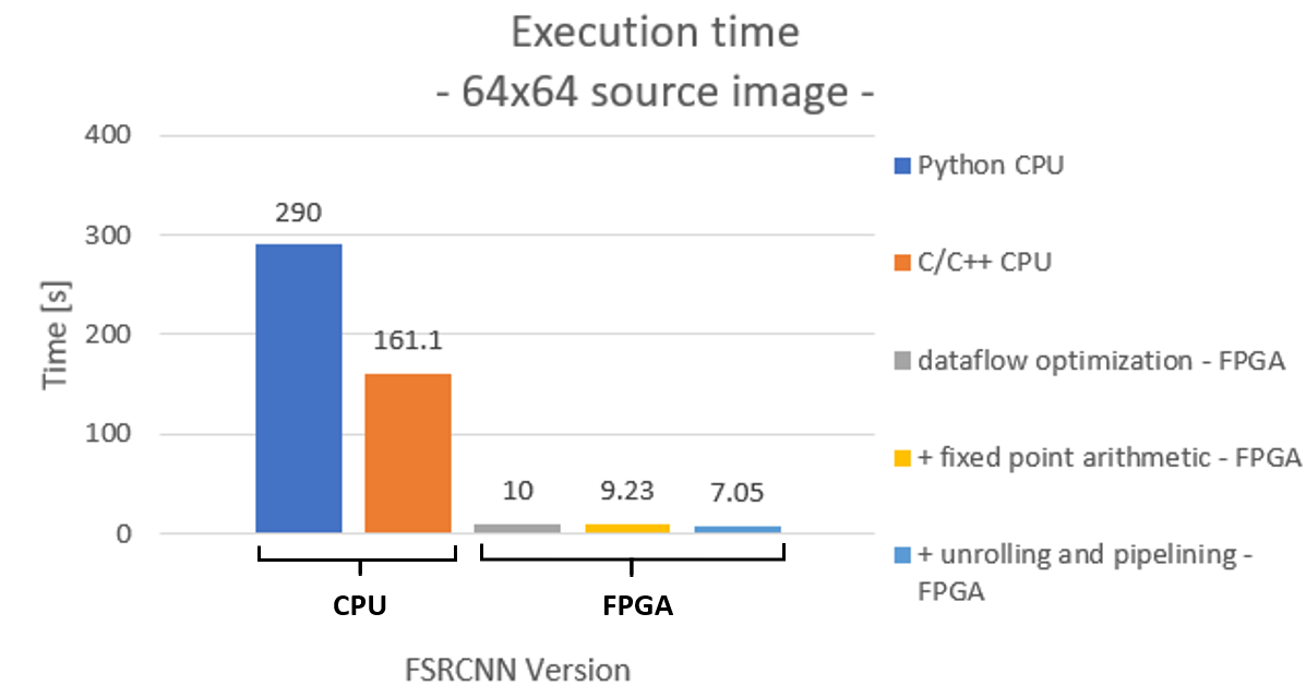
Figures 4 and 5 show the execution times obtained after doubling a 64×64 and a 256×256 source image with different versions of the algorithms I implemented. The FSRCNN FPGA accelerator involves all the acceleration methods I described previously and stands out with a 7.05 seconds runtime for a 64×64 source image. Thus the acceleration factor obtained over the FSRCNN Python version running on a CPU is 41.13X.
 |
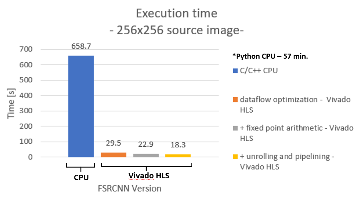 |
Figure 4: FRCNN execution time (upscaling factor = 2)
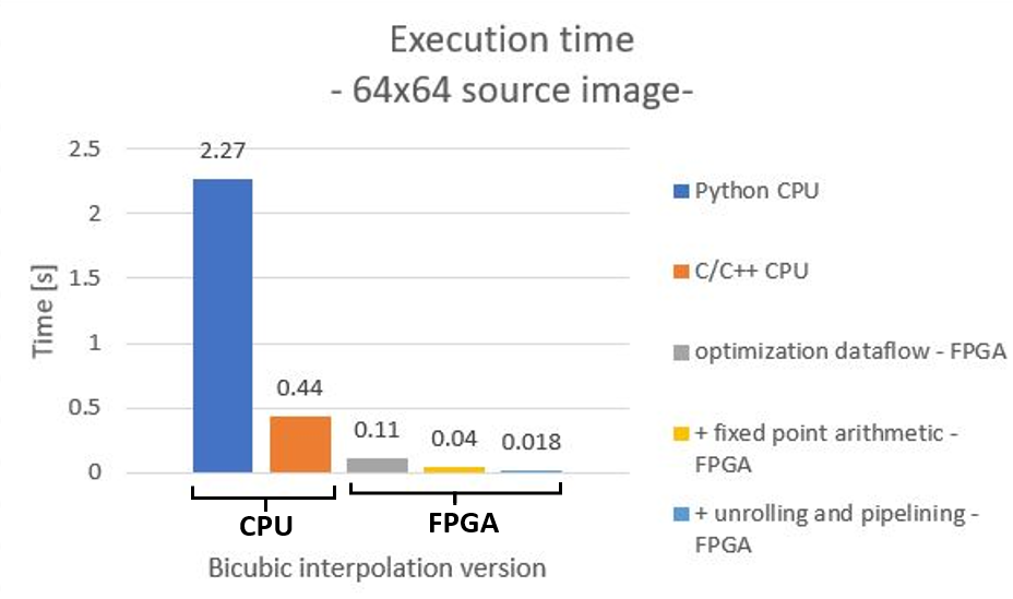 |
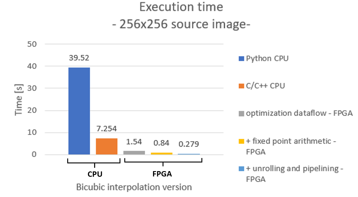 |
Figure 5: Bicubic interpolation execution time (upscaling factor = 2)
Quality Comparison
Stimulating the upscaling images methods with Set5 dataset 64×64 butterfly image, the 128×128 high-resolution images from Figure 6 are obtained. The 64×64 butterfly source image is obtained from downscaling the 128×128 (A) image.
 |
 |
 |
 |
 |
| (A) – reference image | (B) – bicubic interpolation CPU | (C) – bicubic interpolation FPGA | (D) – FSRCNN FPGA | (E) – FSRCNN CPU |
Figure 6: CPU vs FPGA – 64×64 source image and upscaling factor = 2
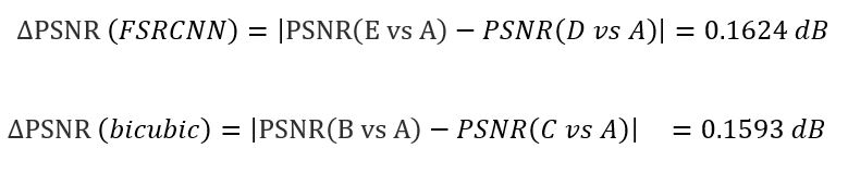
The FPGA uses 24-bit fixed point format variables, as opposed to the CPU which uses 64-bit variables of type double. This is what gives us the differences between the CPU output images and the FPGA output images. In terms of image quality, both the frequency and visual analysis confirm that the images obtained after running on the CPU do not differ significantly from those obtained after running on FPGA. This is confirmed by obtaining a very small ∆PSNR, as it can be seen in the following equations:
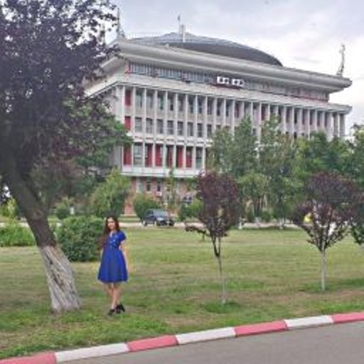
I also analyzed the quality of the results in the case of a personalized image with me in front of the Rectorate building of the Polytechnic University of Bucharest. The upscaled image has 512×512 size. As seen in Figure 7: CPU vs FPGA – 256×256 source image and upscaling factor = 2, the details of the rectorate, the bush behind me, the outline of the dress, as well as the car in the distance are more accurate in images (D) and (E). Images (B) and (C) appear blurred and many details seem lost.
 |
 |
 |
 |
 |
| (A) – reference image | (B) – bicubic interpolation CPU | (C) – bicubic interpolation FPGA | (D) – FSRCNN FPGA | (E) – FSRCNN CPU |
Figure 7: CPU vs FPGA – 256×256 source image and upscaling factor = 2
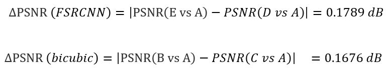
Even in this case, the quality is not significantly lost by porting the algorithms on FPGA, as it can be seen in the following equations:
Conclusion
Throughout this article I have illustrated the following aspects:
- Acceleration of the FSRCNN network on FPGA, reducing the execution time by 22.85X compared to the C/C++ implementation of the network running on the Intel Core i5-6200U X64 CPU, for a 64×64 source image and an upscaling factor = 2;
- An FSRCNN network accelerator emulated in Vivado HLS that reduces the execution time by 36X compared to the C/C ++ implementation of the network running on the Intel Core i5-6200U X64 CPU, for a 256×256 source image and an upscaling factor = 2;
- Acceleration on FPGA, with a negligible loss of magnified image quality;
- An analysis of the execution time-quality trade-off. The bicubic algorithm is faster than the FSRCNN network. However, in the case of interpolation, the upscaled image is more blurred and the cutting artifact is observed, unlike the machine learning method which provides sharp results with more details and greater contrast.
Reproducing the Results
Tools used:
- Operating System: Windows 10
- Simulate, Synthesize, Cosimulate accelerator: Vivado HLS 2019.1
- Block diagram: Vivado 2019.1
- The initial algorithms are tested with the following hardware platform: x64 CPU – Intel Core i5-6200U
- The accelerators are tested with the following hardware platform: Xilinx – Zynq-7000 SoC
To reproduce the results and to find out more details about the accelerator’s implementation, you can read the README files from AMIQ’s GitHub repository.
GitHub
You can download the source code for this project from AMIQ’s GitHub repository.
Acknowledgment
This article is based on my bachelor’s degree project which was accomplished with the guidance of AMIQ Consulting.
Enjoy!
One Response
Hi, this is an excellent project. When I tried to run vitis hls on the run_vitis.tcl, compilation errors out due to opencv2 header file. How did you overcome this?