A Coverage Closure Study: “on-the-fly” or “top-down” Generation?

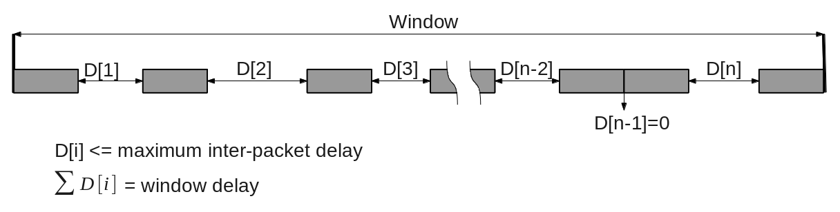
Recently, I’ve verified how a DUT tolerates inter-packet delays. Basically, I’ve driven a fixed number of packets with the following constraints:

• Each inter-packet delay must not exceed a maximum inter-packet delay value
• The sum of all inter-packet delays must be equal with a specified window delay value

At first glance, the most interesting cases appear to be those in which most packets are driven at the begining or at the end of the window, eventually back to back. However, because I don’t have any knowledge about DUT’s internals, I have to make sure I cover all possible scenarios.

For example, if I have to drive 10 packets with maximum inter-packet delay of 3 and window delay of 15, there are 27876 scenarios. In terms of functional coverage implementation, out of 262144 combinations of 9 inter-packet delays (physical space), only 27876 combinations fit the window delay of 15 (valid space).

What I am going to do is searching for a solution to generate random packet sequences that cover all possible scenarios in a reasonable amount of time. For this purpose, I will choose two approaches and then compare them:

1. On-the-fly: generate inter-packet delay before driving each packet
2. Top-down: generate all inter-packet delays up-front and use them when driving each packet

In both cases, I am going to define a sequence of packets with the following properties:

class ..._seq extends uvm_sequence #(packet); 
  //number of packets
  rand int unsigned nof_packets;
  //maximum inter-packet delay
  rand int unsigned max_delay;
  //window delay
  rand int unsigned window_delay;
  ...
endclass

Every packet has a delay property which represents the amount of time to wait before driving the packet. The sequence above always drives the first packet immediately (first packet delay is zero).

class packet extends uvm_sequence_item; 
  // wait delay before driving
  rand int delay;
  ...
endclass

On-the-fly Inter-Packet Delay Generation

An on-the-fly sequence generates the inter-packet delay before driving each packet.

class on_the_fly_seq extends uvm_sequence #(packet);
  ...
  task body();
    // holds the generated delays
    int inter_packet_delay[nof_packets-1];

    // first packet is driven immediately
    `uvm_do_with (req, {req.delay == 0;});

    // for the rest, generate delay before driving the packet
    for(int i = 1; i < nof_packets; i++)begin
      // available delay
      int available_window_delay = window_delay - inter_packet_delay.sum();
      // if not enough delay is used early, 
      // we may end with too much available delay for later packets
      int min_delay = available_window_delay - max_delay*(nof_packets-i-1);

      assert(randomize(new_delay) with {
        // legal delay between 0 and max delay
        new_delay inside {[0:max_delay]};
        // at least minimum delay
        new_delay >= min_delay;
        // at most available window delay
        new_delay <= available_window_delay;             
      });

      inter_packet_delay[i-1] = new_delay;

      `uvm_do_with (req, {req.delay == inter_packet_delay[i-1];}); 
    end
  endtask
endclass

Top-down Inter-Packet Delay Generation

A top-down sequence generates all inter-packet delays up-front:

class top_down_seq extends uvm_sequence #(packet);
  ...
  task body();
    // holds the generated delays
    int inter_packet_delay[nof_packets-1];
      
    // first packet is driven immediately
    `uvm_do_with ( req,{req.delay == 0;});

    // generate delays up-front
    assert(randomize(inter_packet_delay) with {
      // sum of all inter-packet delays equal to window delay
      inter_packet_delay.sum() == window_delay;

      // legal delay between 0 and max delay
      foreach(inter_packet_delay[i])
        inter_packet_delay[i] inside {[0:max_delay]};
    });

    // drive the rest of the packets
    for(int i = 1; i < nof_packets; i++)begin
      `uvm_do_with ( req,{req.delay == inter_packet_delay[i-1];});
    end
  endtask
endclass

Coverage Closure – maximum inter-packet delay 3, window delay 15

The valid space size is 27876.
The charts below show the coverage progress for three simulators when driving 10 packets with maximum inter-packet delay 3 and window delay 15.

On-the-fly

• Simulator 1: 100% after 640k samples
• Simulator 2: 100% after 560k samples
• Simulator 3: 100% after 560k samples

Top-down

• Simulator 1: 99% in 1M samples – Coverage closure is more efficient using on-the-fly generation.
• Simulator 2: 100% after 250k samples – Coverage closure is more efficient using top-down generation.
• Simulator 3: 100% after 470k samples

In the best case, the number of generation cycles required to fill the coverage is 10 times the size of the valid space.

Coverage Closure – maximum inter-packet delay 4, window delay 20

The valid space size is 162585.
The charts below show the coverage progress for the same three simulators when driving 10 packets with maximum inter-packet delay 4 and window delay 20.

On-the-fly

• Simulator 1: 97% after 1M samples
• Simulator 2: 97% after 1M samples
• Simulator 3: 97% after 1M samples

Top-down

• Simulator 1: 79% in 1M samples – Coverage closure is more efficient using on-the-fly generation.
• Simulator 2: 99.8% after 1M samples – Coverage closure is more efficient using top-down generation.
• Simulator 3: 99.3% after 1M samples – Coverage closure is more efficient using top-down generation.

Conclusions

Top-down or On-the-fly

Intuitively, I’ve expected the top-down approach to be more efficient, because all the constraints are specified directly on the generated list, and a generator could uniformly spread values in the valid space. However, this is not true for all simulators. Simulator 1 above does not fill coverage faster in a top-down approach.

Coverage Closure Benchmarks

Simulator 2 seems to be more efficient in terms of coverage progress. It needs fewer samples to reach boundaries like 80%, 90% or 100%, especially using the top-down approach.

Since the intriguing question has always been whether the simulation speed is the only criteria for choosing a simulator, perhaps we should take into consideration the coverage closure speed, as coverage closure is something we look for, when doing verification.

One may say that bugs linger around, not necessarily pinpointed by coverage samples, and filling coverage slower raises the probability of hitting unexpected corner cases. A slower coverage closure simulator may prove beneficial for discovering bugs.

However, the verification process should be controllable; the verification plan describes interesting scenarios that should be covered, and that’s why we spend a lot of time filling coverage. I believe that one should consider coverage closure speed when it comes to choosing a simulator.

I wonder: what should be the coverage closure benchmarks for measuring a simulator performance?